Blog | Turning Gini into Profits

Written by Rodrigo Sanabria, Director Partner Success, Latin America

On a prior post by Carlos del Carpio (“The Economics of Credit Scoring”), we discussed the business considerations to assess the merit of a risk model. In this post, I will address how a good origination model impacts the bottom line of a company’s P&L.

These principles may be adapted to look into other types of models used at later stages of a loan life, but on this post we will only address loan origination.

From a business point of view, an origination model is a tool that helps us aim at the “sweet spot”: where we maximize profits. A simple way to think about it is as a trade-off between the cost of acquisition (per loan disbursed) and cost of defaults (provisions, write-offs): The higher the approval rate, the lower the cost of acquisition, but the number of defaults go up.

How do we go about finding the sweet spot? I’ll try to explain it below.

Figure 1

A good model has a good Gini. A “USEFUL” model creates a steep probability of default (also known as PD) curve – we usually refer to it as a “risk split”.

Figure 1 shows the performance of a model based on psychometric information used by an MFI. The Gini (not shown in the graphic) is pretty good (0.28). The risk split is great: the people in the lower 20% of the score ranking are about 9 times more likely to default than those in the top 20%.

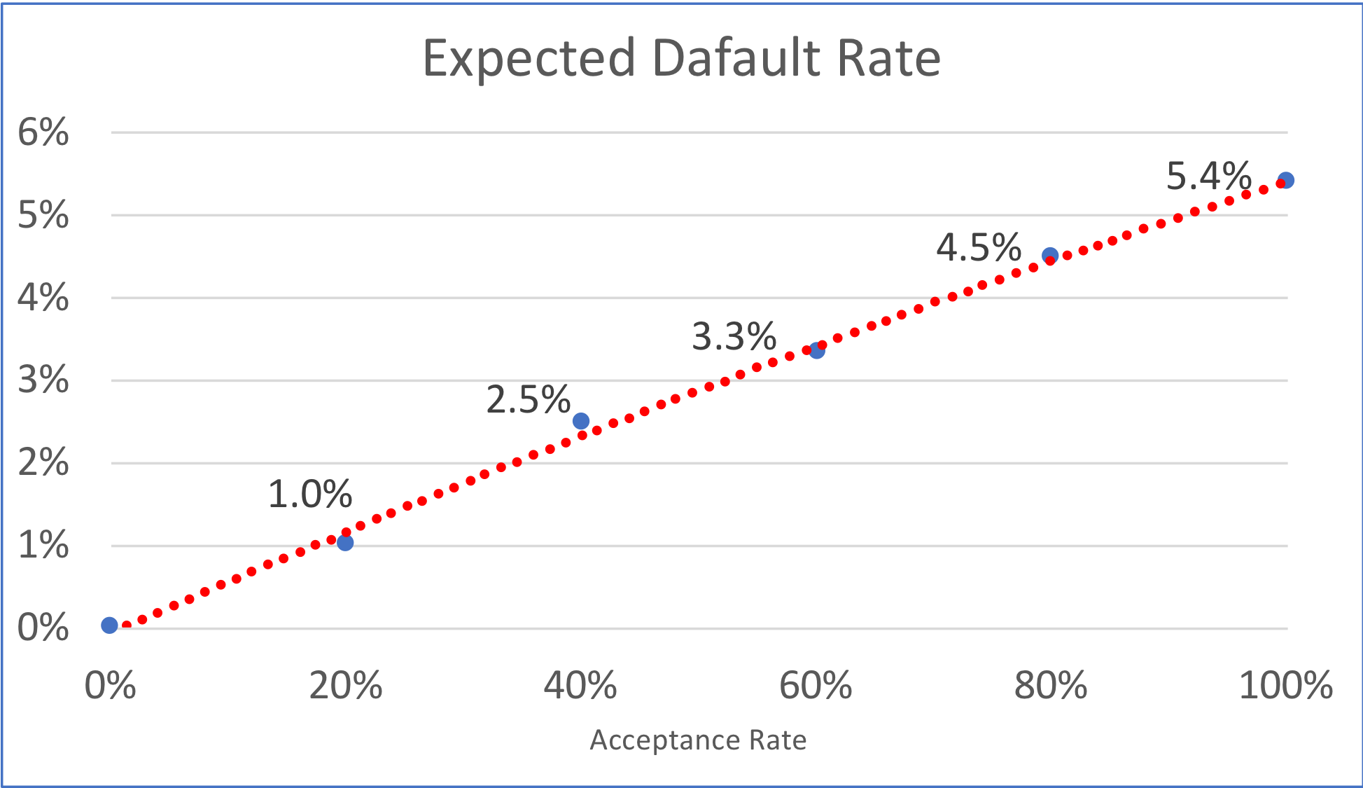
Knowing the probability of default for a given group, we may set a credit policy. Basically, we need to answer: “what would the default look like given an acceptance rate?”

Figure 2

We have re-plotted the same data in Figure 2, but now we express the probability of default in accumulated terms. Basically, the graph shows that if we were to accept 80% of this population sample, we would have a 4.5% PD, but if we were to accept 40%, the PD would go down 2 points to 2.5%.

Now, from a business point of view, we still do not have enough information to decide. Do we?

Where would the profit be maximized?

The total cost of customer acquisition is mainly fixed. Whatever we spend on marketing and sales to attract this population, will not change if we reject more or fewer applicants. So, the cost per loan disbursed would grow as we reduce the acceptance rate.

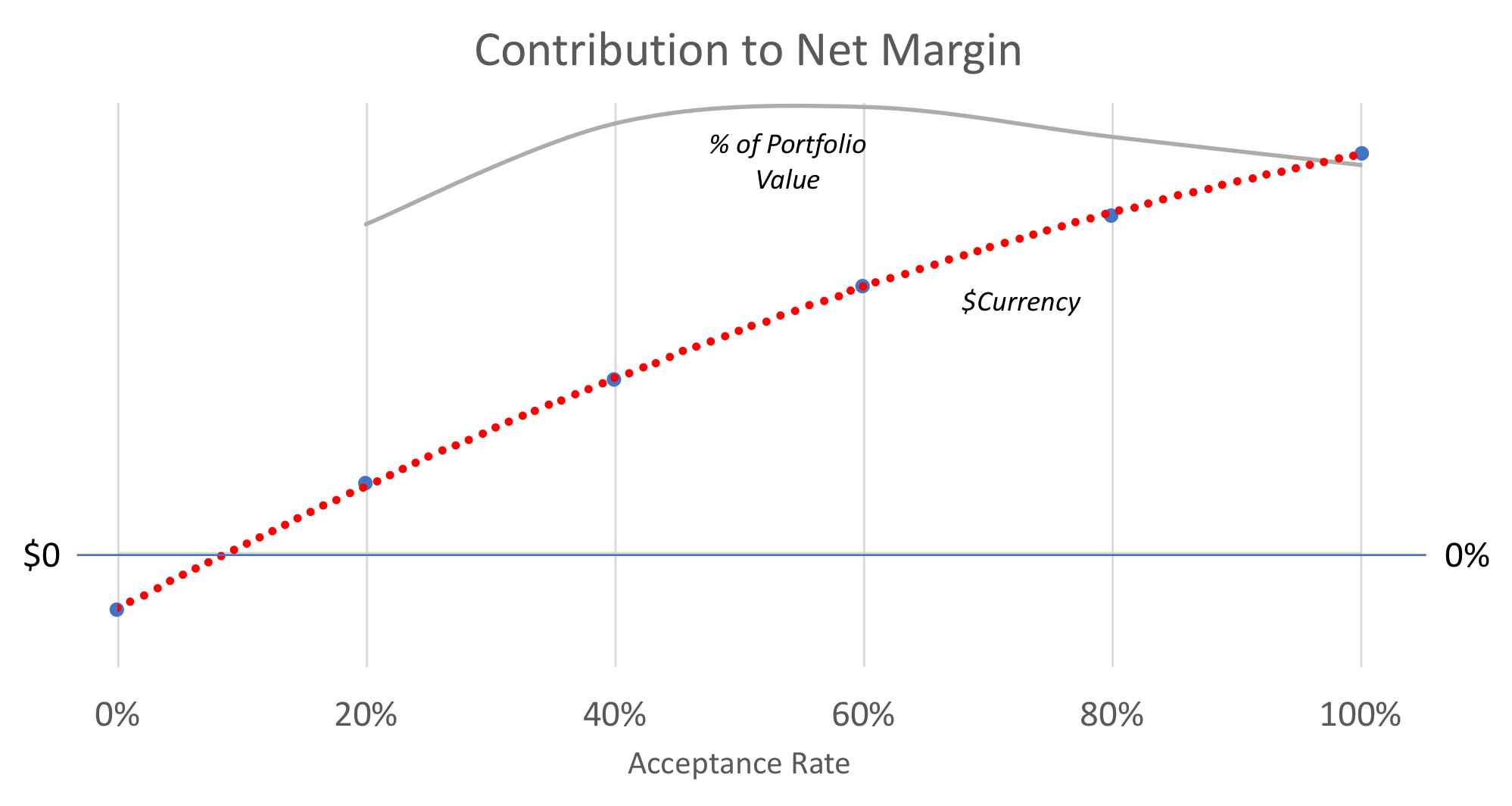
Of course, the higher the acceptance rate, the larger the portfolio, and the more interest revenue we get. BUT, the higher the provisions and write-offs. The combination of these 2 variables (cost of acquisition and net interest income) produces an inverted U-shaped curve that uncovers the “sweet spot”

Figure 3

The current credit policy is yielding a profit at 100% acceptance rate (see Figure 3) because the sample being analyzed corresponds to all the customers that were accepted (i.e. we have repayment data about them). So, the portfolio is profitable.

But the sweet spot seems to be shy of 60% acceptance rate. If this FI were to cut down its approval rate to that level, profits would increase by about a third, and its return on portfolio value would almost double. Of course, there are other considerations around market share and capital adequacy that may play a role in such a strategic decision, but the opportunity is clearly uncovered by the model.

In my experience, the sweet spot usually lies within 30%-70% acceptance rates, driven by marketing expenditures, interest rates, cost of capital, sales channels, and regulation.

What if the shape of the curve shows a continuous positive growth? The sweet spot is at a 100% acceptance rate! – have we reached risk karma? – Most likely, the answer is no (but almost!).

Figure 4

Most likely, we are leaving money on the table. Some business rule may be filtering people before they are scored. I have experienced this situation while working with lenders. For example, a traditional bank was filtering out all SMEs that had been operating for less than X years. This bias in the population was creating a great portfolio from a PD point of view, but there was clearly an opportunity to include younger businesses. As you can see in Figure 4, the maximum return on the portfolio was achieved at 60% approval rate, but they could increase profits by approving beyond the current acceptance rate. Depending on their cost of capital, it may be a good idea to expand the portfolio by approving more people.

In summary, think of your origination model as a business tool. Don’t stop at looking at Gini to assess a model’s merit. Understand how your profitability would be impacted by changes in your acceptance rate. If the PD curve is steep enough, you may capture quite a lot of value by applying the model to either reduce or increase your acceptance rate.

Blog | On the use (and misuse) of Gini Coefficients in Credit Scoring: the Economics of Credit Scoring

This is the fourth part of a series of blog posts about Ginis in Credit Scoring. See also part 1, part 2, part 3.

Gini Coefficients and the Economics of Credit Scoring

On a global scale, billions of dollars in debt are granted every year using decisions derived from credit scoring systems. Financial institutions critically depend on these quantitative decision to enable accurate risk assessments for their lending business. In this sense, as with any tool that serves a business purpose, the application of credit scoring is not ultimately measured by its statistical properties, but by its impact in business results: how much can Credit Scoring help to increase the benefit and/or to decrease the cost of the lending business.

Assessing Credit Scoring from a business perspective could sound pretty obvious. However, given the typical compartmentalization of roles that could exist at lending institutions, where Risk and Modeling teams can be completely separated from Commercial departments, it could be easy sometimes to focus too much on the statistical aspects of credit scoring such as Ginis, and forget the ultimate business nature of its purpose. Although there is a clear positive relationship between economic benefits and predictive power, there are also certain elements that can affect the balance between costs and benefits. In this post, we discuss some of these elements and explain their role in the cost-benefit analysis of credit scoring.

The benefits of credit scoring

The benefit of credit scoring derives from its ability to accurately identify good customers, and discriminate them from bad customers. The more good customers a model can identify, the greater the interest income that can be generated from a credit portfolio. And the more bad customers it can discriminate, the lower the losses for the credit portfolio. In this sense, the economic benefit of credit scoring can be amplified by two things: the volume of customers, and the size of the credit disbursed to these customers.

Take for example the portfolio of microfinance institution “A” with several thousands of customers but very small loan amounts, and compare it against a smaller microfinance institution “B” providing loans of the same size to a portfolio of just a few hundred customers. Both institutions can see a similar increase of 1% in the predictive power of their credit scoring models, however, the increase in economic benefit yielded from this increase in predictive power will be different just because of the different sizes of portfolio volumes. Everything else being equal, the higher the volume of the portfolio, the higher the potential economic benefit of credit scoring.

The same can be argued for the size of credit disbursed to the customers of a portfolio. For example, take an SME lending institution with just a few thousands of customers but with relatively high credit amounts in the hundreds of thousands of dollars. An increase of 1% in predictive power could bring just a handful of new good clients into the portfolio, or avoid the disbursement of a handful of very bad loans. However a change in just a handful of good or bad clients can be enough to generate a considerable increase of economic benefit in the portfolio given the large size of the loans.

The costs of credit scoring

The costs of Credit Scoring can be split in two parts. First, the cost of developing a new model, and secondly, the cost of implementing and maintaining credit scoring models.

If we assume lending institutions are at a stage of technological maturity in which all the necessary data to create a credit scoring model exists and is continuously updated with certain level of quality and integrity, then the first type of cost just depends on the complexity of the modeling process. The whole process of building a model includes data extraction and cleaning, feature engineering, feature selection and the selection of a classification algorithm.

Depending on the lending institution, this process can be handled by a single data scientist (e.g. think of the CRO of a small Fintech startup), or it can be handled by a large department including many different teams with different roles such as data engineers, data scientists and software engineers (e.g. think of a large multinational bank). At the same time, the teams in charge of the model building process can be comprised of junior analysts fresh out of college using well-known standard techniques or include teams of PhDs in computer science doing advanced machine learning. At the end, the cost involved in developing the credit scoring models will depend on how much complexity and sophistication can be afforded and/or needs to be put into the process.

Once the model has been built, it also needs to be implemented and monitored over time. The costs involved are not trivial. Again, they will depend on the stage of technological maturity of the financial institution and the complexity and sophistication required. For example, in some cases the implementation of a credit scoring model can be as simple as creating an Excel calculator loaded with the coefficients of a logistic regressions where some values are manually inputted by a Loan Officer to get a score (e.g. think of a small MFI in the rural area of a developing country). Or it can be as complex as a Python package in a cloud-hosted decision engine integrated in the online platform of a large bank. The handling of big data, software development and testing, as well as the security and legal aspects involved in the deployment of a credit scoring system can considerably increase its costs. And all this, without even considering if the teams that will monitor the performance of the models implemented on a defined frequency basis are dedicated full time, or they are just the same team that also did the modeling and/or deployment.

Bottom-line:  The statistical classification accuracy measured by Gini coefficients are indicative of some part of the benefits of using credit scores, but they are not the most important nor the final metric when assessing the cost-benefit of credit scoring. The reason is because the benefits of credit scoring can be influenced by the volumes of customers and the size of the credit. And the costs of credit scoring ultimately depends on the stage of technological maturity of the lending institution, as well as how much complexity and sophistication can be afforded and need to be put in the development, deployment and monitoring of credit scoring models.   

So next time you need to make a decision about using Credit Scores to boost your lending business, ask how much they can help to increase the benefits of the business, and how much they can help to decrease its cost. The final decision will depend on a lot more than just Ginis.

At LenddoEFL, we have the expertise to help you boost the benefits and reduce the costs of credit scoring using traditional and alternative data. Contact us for more information here: https://include1billion.com/contact/.

Blog | On the use (and misuse) of Gini Coefficients in Credit Scoring: Comparing Ginis

By: Carlos Del Carpio, Director of Risk and Analytics, LenddoEFL

This is part 2 of a series of blog posts about Ginis in Credit Scoring. To see the part 1, follow this link.

What is an AUC?

AUC stands for “Area Under the (ROC) Curve”. From a statistical perspective, it measures the probability that a good client chosen randomly has a score higher than a bad client chosen randomly. In that sense, AUC is a statistical measure widely used in many industries and fields across academia to compare the predictive power of two or more different statistical classification models over the exact same data sample [1].

How is AUC used in Credit Scoring?

In the particular case of Credit Scoring, AUCs are useful for example in the model development process, when there are several candidate models built over the same training data and they need to be compared. Another typical use is at the time of introducing a new credit score, to compare a challenger against an incumbent score over the same sample of data under a champion challenger framework.

How does AUC relate to Gini Coefficient?

The Gini Coefficient is a direct conversion from AUC through a simple formula: Gini = (AUC x 2) -1. They measure exactly the same. And it is possible to go directly from one measure to the other, back and forth. The only reason to use Gini over AUC is the improvement in the scale’s interpretability: while the scale of a good predicting model AUC goes from 0.5 to 1, the scale in the case of Gini goes from 0 to 1. However, all the properties and restrictions of AUC still translate into Gini Coefficient, and this includes the need to compare two different AUC values over the exact same data sample to make any conclusion about their relative predictive power.

What does this mean in practical terms?

Any direct comparison of the Gini Coefficients (or AUCs) of two different models over two different data samples will be misleading. For example: If a Bank A has a Credit Score with a Gini Coefficient of 30%, and Bank B has a Credit Score with a Gini Coefficient of 28%, it is not possible to make any conclusion about which is better or which is more predictive because they have been calculated over different data samples without accounting for the difference in absolute number of observations and the difference in proportion of good cases against bad cases. The only direct comparison possible is the one made about two scores side by side, over the exact same data sample.

Bottom-line: To affirm that a certain absolute level of AUC or Gini Coefficient is “good” or “bad” is meaningless. Such affirmation is only possible in relative terms, when comparing two or more different scores over the exact same data sample. Unfortunately this is often not well understood, which leads to the most frequent misuse of AUC and Gini Coefficients, such as direct, un-weighted comparisons of Gini values across different samples, different time periods, different products, different segments and even different financial institutions.

[1] Hanley JA, McNeil BJ. The meaning and use of the area under a Receiver Operating Characteristic (ROC) curve. Radiology, 1982, 143, 29-36.

Blog | On the use (and misuse) of Gini Coefficients in Credit Scoring

Over years of blogging, one of our most popular ever blog posts was about the Gini coefficient. In this series of posts, we revisit the Gini and dig further into its uses and the ways we see it misused in credit scoring.

What is a GINI?

For lenders around the world, the “Gini Coefficient” is an often heard, sometimes feared, and frequently misunderstood statistical measure. Commonly used to assess things like wealth inequality, Gini Coefficients are also used to evaluate the predictive power of credit scoring models. In other words, a Gini Coefficient can help measure how good a credit score is at predicting who will repay and who will default on a loan: the better a credit score, the better it should be at giving lower scores to riskier applicants, and higher scores to safer applicants.

Though calculating a Gini Coefficient is complex, understanding it is fairly simple:

A Gini Coefficient is merely a scale of predictive power from 0 to 1, and a higher Gini means more predictive power.

However, there are a few key aspects of Gini Coefficients that are not always well understood and can lead to their misuse and wrong interpretation. Over this series of blog posts we’ll discuss four of them:

1. People often compare Ginis when they should not. The only useful comparison across Ginis (or AUCs) is when looking at different scores over the exact same data. 

2. People forget that Gini will vary by acceptance rate. When presented with a Gini coefficient, always keep an eye on the effect of the acceptance rate.

3. People focus on Ginis, but are not always aware of its impact on the costs, benefits and overall economics of Credit Scoring.

4. People do not fully understand and often overestimate the role of Gini in the business of lending.

About the Author:

Carlos del Carpio is Director of Risk & Analytics at LenddoEFL. He has 10+ years of experience developing credit scoring models and implementing end-to-end credit risk solutions for Banks, Retailers, and Microfinance Institutions across 27+ countries in Latin America, Asia and Africa.

About LenddoEFL

LenddoEFL’s mission is to provide one billion people access to powerful financial products at a lower cost, faster and more conveniently. We use AI and advanced analytics to bring together the best sources of digital and behavioural data to help lenders in emerging markets make data-driven decisions and confidently serve underbanked people and small businesses. To date, LenddoEFL has provided credit scoring, verification and insights products to over 50 financial institutions, serving seven million people and lending two billion USD. For inquiries about our products or services please contact us here.

Blog | Raising the Stakes on Psychometric Credit Scoring

An updated and expanded 2nd edition (first edition)

Why read this post?

Learn why high-stakes data is essential for building accurate credit-scoring models.

Introduction

Billions of people lack traditional credit histories, but every single person on the planet has attitudes, beliefs, and behaviors that can be used to predict creditworthiness. Quantifying these human traits is the focus of psychometrics, and the alternative data provided by this technique allows LenddoEFL to greatly expand financial inclusion in its mission to #include1billion.

But there is a catch: in order to build models that accurately predict default, applicants need to complete psychometric assessments in pursuit of actual financial products, a so-called “high-stakes” environment. This is because people answer psychometric questions differently when they have a chance to receive a loan (the high stakes) than they would in a hypothetical situation with no incentive (the low stakes).

Despite this fact, psychometric tools are frequently built using low-stakes data. For example, many companies develop psychometric credit scoring tools using volunteers. And many lenders want to validate psychometric credit scoring tools on their clients through back-testing: giving the application to existing clients and comparing scores to their repayment history, again a low-stakes setting.

These approaches are only valid if low-stakes data can be applied to the real world of high-stakes implementation, where access to finance is on the line for applicants. But it turns out that this is not the case. A recent study published by our co-founder Bailey Klinger and academic researchers proved that low-stakes testing has no predictive validity for building and validating psychometric credit scoring models in a real-world, high-stakes situation. The data below shows exactly how applicant responses shift as they move from one environment to another.

 

The Experiment

To test for differences between low- and high-stakes situations, LenddoEFL gathered psychometric data from two sets of micro-enterprise owners in the same east-African country. One group already had their loans (low-stakes) and another group completed a psychometric assessment as a part of the loan application process (high-stakes).

First, the low-stakes data. The figure below shows the frequency distribution for two of the most important ‘Big 5’ personality dimensions for entrepreneurs, Extraversion and Conscientiousness, as well as a leading integrity assessment[i].
 

You can see that when the stakes are high, people are answering the same questions very differently. The distribution of scores on these three personality measures shifts significantly to the right. When something important is at stake, like being accepted or rejected for a loan, people answer differently.

How do these differences in low- vs. high-stakes data matter for credit scoring?

To see how these differences impact the predictive value of psychometric credit scoring, we can make two models[ii] to predict default: one uses responses from applicants that took the application in low stakes settings, and the other uses responses from applicants that were in high stakes settings. Then we can use a Gini Coefficient—which measures the ability of a model to successfully rank-order applicants’ riskiness and for which a higher coefficient is a metric of success in this—to compare each model’s ability to predict default for the opposing population as well as its own.[iii]

These results clearly show that there is a significant change in the rank ordering when models built on low-stakes data are applied in high-stakes settings and vice versa.[iv] Importantly, we can see that a psychometric credit-scoring model can indeed achieve reasonable predictive power in a real-world, high-stakes setting. But, that is only when the model was built with high-stakes data.

Think about it like this: when the stakes are high, both less and more risky applicants change their answers. But, less risky applicants change their answers in a different way than riskier applicants. This difference is what is used to predict risk in psychometric credit scoring models: the difference between how low- and high-risk people answer in a high-stakes setting.

This also illustrates why we see that a model built on low-stakes data is ineffective in a real-world high-stakes implementation. In the low-stakes setting, the low- and high-risk people aren’t trying to change their answers, because they aren’t concerned with the outcome of the test. Once the stakes are high, however, this pattern changes.

 

Conclusions

Testing existing loan clients or volunteers has an obvious attraction: speed. That way you don’t have to bother new loan applicants with additional questions, and then wait for them to either repay or default on their loans before you have the data to make or validate a score, an approach that takes years.

Unfortunately, these results clearly show that this shortcut does not work. People change their answers when the stakes are high, so a model built on low-stakes data falls apart when used in the real-world. People answer optional surveys with less attention and less strategy than they do a high-stakes application, and therefore the only strong foundation to a predictive credit-scoring model is real high-stakes application data and subsequent loan repayment.

Consider an analogy: you can’t predict who is a good driver based on how they play a driving video game, where the outcome is not important. Conversely, someone who does well on a real-world driving test may not perform that well on a video game.  Whether it is driving skills or creditworthiness, you must predict the high-stakes context with high-stakes data.

TAKEAWAYS:

- Psychometric model accuracy is only guaranteed when you collect data in a high-stakes situation (i.e., a real loan application).

- Despite its speed, back-testing a model on existing clients in a low-stakes setting is risky because it might not tell you anything about how the model will work in a real implementation.

- If you want to buy a model from a provider, the first thing you should verify is what kind of data they used to make their model. Was it from a real-world high-stakes implementation similar to your own?

[i] These are indices from widely available commercial psychometrics providers. It is important to note that LenddoEFL no longer uses any of these assessments or dimensions in our assessment, nor any index measures of personality.

[ii] Stepwise logistic regression built on a random 80% of data, and tested on the remaining 20% hold-out sample. An equivalently-sized random sample was used from the other set (high-stakes data for the low-stakes model, and low-stake data for the high-stakes model) to remove any effects of sample size on gini.

[iii] Note that this exercise was restricted to those questions that were present in both the low- and high-stakes testing. It does not represent LenddoEFL’s full set of content and level of predictive power, it is only for purposes of comparing relative predictive power.

[iv] The results also show that using standard personality items, the absolute predictive power is lower in a high-stakes setting compared to a low-stakes setting. This is likely because of the ability to manipulate some items in a high-stakes setting makes them not useful within a high-stakes setting. This lesson has lead LenddoEFL to develop a large set of application content that is more resistant to manipulation and which has much higher predictive power in high-stakes models. This content forms the backbone of the current LenddoEFL psychometric assessment, all of which is built and tested exclusively with high-stakes data and subsequent loan repayment-default rather than back-testing.